Masked Non-negative Matrix Factorization
Introduction
Non-negative matrix factorization is a powerful tool for dimensionality reduction and data analysis. The goal in matrix factorization, in general, is to summarize a given data matrix with two low-rank factors. In this non-negative matrix factorization (NMF), we require the factor matrices to have only non-negative elements. This is in contrast to some other factorization methods, such as principle component analysis (PCA). In this brief article, we are interested in scenarios where not all the elements in the given data matrix are measured or valid. In this case, we want to "skip" these missing elements when solving the optimization problem and find the factor matrices without considering the error on those elements.
The non-negative matrix factorization problem
Given the non-negative data matrix we want to find matrices and such that . The optimization problem can be written as
An iterative algorithm
The following algorithm, called Lee and Seung's multiplicative update rule, solves the NMF problem.
initialize: W and H with random non-negative elements
repeat until convergence:
One drawback of this algorithm is that when an entry of or is initialized as zero or positive, it remains zero or positive throughout the iterations. Therefore, all entries should be initialized to be positive and sparsity constraints are not simply added to the algorithm unless via hard-thresholding.
Alternating non-negative least squares algorithm
Another algorithmic solution can be achieved via alternating non-negative least squares (ANLS). Assume we have fixed then we get the following optimization for :
which is the least squares problem for with a non-negativity constraint. The solution to this problem can be determined by solving for followed by a projection onto . We can also use the method proposed in this paper to solve this problem. The code can be found here. Now for fixed we can write:
This can be minimized by solving for , followed by the projection onto . It is also recommended that we normalize the columns of to unit -norm and scale the rows of accordingly after each iteration. Using changes in per iteration, we can define the stopping criteria.
Masked non-negative matrix factorization
In real application, we might have a case where the columns of represent different data-points and each row represents a separate features. In this case, we might have a situation where some of the features are missing from the dataset. In the NMF formulation, we do not want to consider the error over these missing values. In other words, we only wanna consider the error on the elements in that are valid or measured and discard the error on the rest. It is fair to assume that we know which elements are missing and use this information when formulating the problem.
Let be the masking matrix such that iff is missing, otherwise . In this case we only want to consider the error on measured signals. So we get,
where denotes the element-wise multiplication. The loss function in this case only considers the error in elements of where is non-zero.
How do we add the Masking to an iterative solver?
We can apply the ANLS algorithm to the masked problem. When we fix we get the following optimization over ,
Following the ANLS method we have to solve for followed by a projection onto . The derivation here shows the solution without the non-negative constraint. Let where is the -th column of . Then, these equations can be solved for each column of separately by solving the linear system for . We note that this can still be solved by nnlsm_blockpivot.m method from this paper. When an element in is zero, we remove the corresponding row from the linear system (technically there is no need to do this and we can directly form and and solve the linear system, however, by removing the zeros we make sure that does not become unnecessarily ill-conditioned).
Now for fixed we can write:
which is solved by the system of equations for followed by a projection onto . Similarly, this can be diagonalized for rows of the matrix and solved via the same method.
Example: Hubble images with missing pixels
The Hubble images dataset consists of 100 images of the Hubble telescope where each image highlights different materials. For example, five samples of these images are
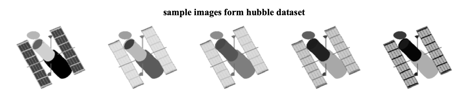
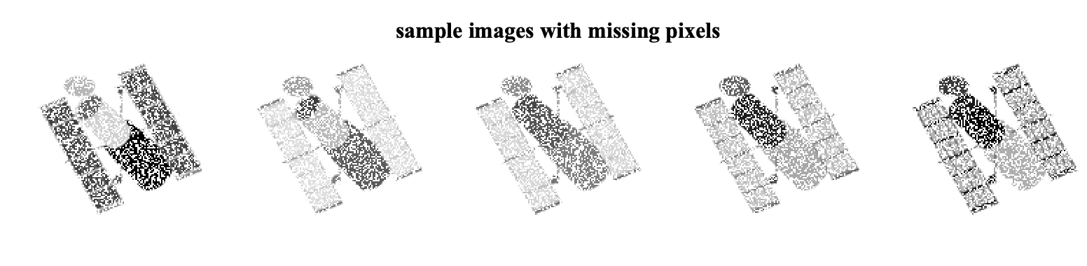
Each image is converted into a column vector and is stored in the our data matrix D. In this case, D is a matrix of size 16384 x 100 (note that each image is 128x128). To simulate the missing pixels, we compute the masking matrix by randomly choosing 60% of the pixels.
D = ... % load from Hubble.mat
% create a random mask -- keep p% of enteries
p = 0.6;
M = rand(size(D))<=p;
% data with missing enteries
MD = M.*D;
The sample images when we set the missing pixels to zero are
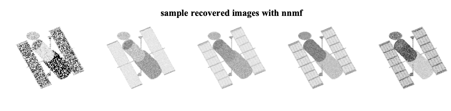
If we just call the nnmf function in Matlab with the matrix MD we get the NMF solution without considering the mask. Lets assume we consider rank to be eight!
% set a rank
r = 8;
% run nnmf without masking
[W_nmf,H_nmf] = nnmf(MD, r);
% recovered estimated data
D_hat_nmf = W_nmf*H_nmf;
The recovered sample images are
Now lets consider the solution via masked-nnmf. In this case, we need to provide the masking matrix M to the solver as well as the desired rank r.
% run the solver
[W,H] = masked_nnmf(MD, M, r,...
                    'init_mode', 'rand',...
                    'maxiter', 250);
% recovered estimated data
D_hat = W*H;
The recovered sample images in this case are
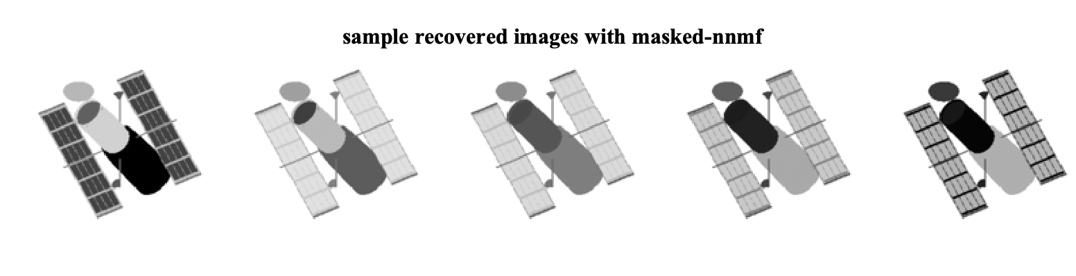
As we can see, by ignoring the missing data, we can exploit the low-rank structure of the original data matrix and recover the missing pixels. We can further look at the factors that are found by each algorithm. Note that the W matrices are of size 16384 x 8 and can be viewed as eight different factor images for each method. The factor images from nnmf and masked-nnmf are
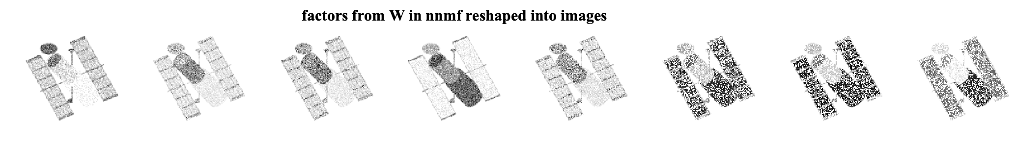
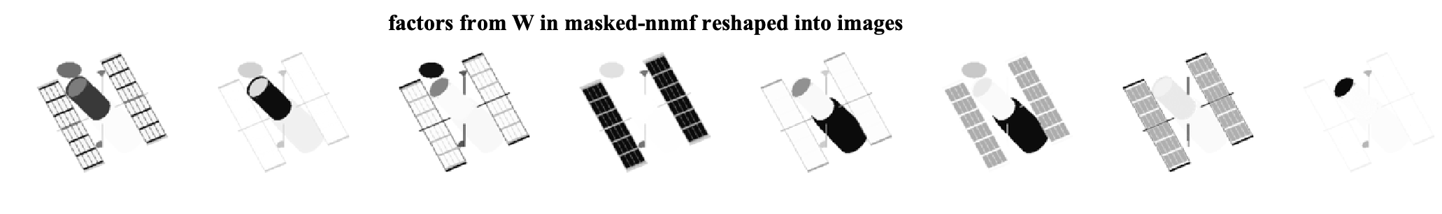
We see that the method considering the masking better finds the underlying low-rank structure.
A note on implementation in Matlab
I implemented this algorithm in Matlab and you can find the code here. The core solver is the masked-nnmf function. Here is a brief overview of the main iteration.
The solver function receives three main inputs:
D: the data matrix of sizem x n.M: the mask matrix of sizem x nwith elementsMij = 0iffDijis missing.r: desired rank.
The main loop consists of an update over followed by an update over . Given the matrix M we can precompute the rows in and that we need to use when solving for . Similarly, we find columns to use in each row of and when solving for rows . We write the update iteration as:
% update H
WT = W';
parfor (j = 1:size(D,2), num_cores) % loop over columns of D
	WT_mj_dj = transpose(sum(W(rows2use{j},:).*D(rows2use{j},j),1));
	WT_mj_W = WT(:,rows2use{j}) * W(rows2use{j},:);
	H(:,j) = nnlsm_blockpivot(WT_mj_W, WT_mj_dj, true);
end

% update W
HT = H';
parfor (i = 1:size(D,1), num_cores) % loop over rows of D
	H_mi_di = sum(H(:,cols2use{i}).*D(i,cols2use{i}),2);
	H_mi_H = H(:,cols2use{i}) * HT(cols2use{i},:);
	W(i,:) = nnlsm_blockpivot(H_mi_H, H_mi_di, true);
end
References
For further reading on the NMF problem with missing data, this paper is a good read!
For the solution of non-negative least squares problem you can take a look at this blog post from Alex Williams.